Haskell data visualization part 1: Hello, plots

I learned Python a decade ago because I visited my partner’s lab when she was working on SPIDER and I saw plots in kst that told her whether one of the machines would explode.¹ I spent all of my formative just-enough-Python-to-be-dangerous time at my first job with pandas, matplotlib, and an assortment of other Python plotting libraries. I hand-rolled tables with shaded cells and abused the annotations and shapes APIs while trying to convince any coworker of mine who hadn’t yet lost patience for that discussion that we should get rid of all of our Stata and SAS and R and Excel² and whatever else people were using and do everything in Python. When I want to plot something now, I’ve often finished typing fix, ax = plt.subplots() before I’ve even figured out what kind of plot I want.

I’m explaining all this because a week ago I got around to posting Don’t fire Styer with some plots showing distributions of simulated outcomes for an annual USA vs. Europe pool event. One of the challenges I set myself while working on that was that I wasn’t allowed to use Python to produce the plots – I had to produce them in Haskell, the same language I used for the simulation code.

I wound up using the built-in plotting utilities of the new-ish Haskell dataframe library, but there are options for Haskell visualization libraries now, and I wanted to know what else is out there.

This post is the first of, I don’t know, probably three or four posts on data visualization in Haskell in early 2026.

Plotting with Haskell Libraries

I found a few libraries, with some help from the DataHaskell Discord.

• dataframe
• granite
• hvega
• Chart
• chart-svg

I wanted to compare them on a few points, starting with what it looks like to take a dataframe and produce a scatter plot. I think of scatter plots as “hello, world” for plotting things.

Each library has its own idea of what kind of data is plottable. I’m starting with a dataframe in every case to hand-wave away some of that difference and to focus instead on getting from some kind of data to some kind of graphic.

I’m not going to pick winners and losers, just comment on what’s easy and difficult at each stage along the way. Especially at this early stage saying one library is better than another would be premature – “it’s easy to do something easy” and “it’s easy to do something hard” are basically uncorrelated.

For each plot, I used a dataframe full of random points in columns x and y. All examples are available in my goofing-off repository.

Without any further ado, here are five scatter plots with code samples.

dataframe

{-# LANGUAGE OverloadedStrings #-}

import qualified Data.Text.IO as Text
import qualified DataFrame as D
import qualified DataFrame.Display.Web.Plot as DfPlot

dataframeScatter :: D.DataFrame -> IO ()
dataframeScatter df =
  DfPlot.plotScatter "x" "y" df
    >>= (\(DfPlot.HtmlPlot plot) -> Text.writeFile "plots/dataframeScatter.html" plot)

dataframe’s built-in plotting is what I used for the previous post. Not surprisingly, its plotFoo functions all take dataframes and column references. I started on this before the new typed module that can make column references type safe, so my references are just text.

The output is an HtmlPlot newtype around Text, so it’s easy to send it to a file, but complicated to transform (more to come on that in part 2).

granite

{-# LANGUAGE OverloadedStrings #-}

import qualified Data.Text.IO as Text
import qualified DataFrame as D
import qualified Granite as G
import qualified Granite.Svg as GSvg

graniteSvgScatter :: D.DataFrame -> IO ()
graniteSvgScatter df =
  let xs = D.extractNumericColumn "x" df
      ys = D.extractNumericColumn "y" df
      plot = GSvg.scatter [G.series "points" (zip xs ys)] G.defPlot
   in Text.writeFile "plots/graniteSvgScatter.html" plot

granite is another library from @mchav, who also owned the dataframe repo before it moved to DataHaskell. It originally focused on terminal plots³, but he added an SVG backend when I mentioned I was working on this in the DataHaskell Discord.

granite doesn’t natively speak dataframes, but it’s easy to get data out in the form that granite wants it, specifically a series of point tuples. While the specifics vary, this is a common theme for the rest of the plotting libraries, so I won’t mention it again.

hvega

{-# LANGUAGE OverloadedStrings #-}

import qualified DataFrame as D
import qualified Graphics.Vega.VegaLite as V

hvegaScatter :: D.DataFrame -> IO ()
hvegaScatter df =
  let vegaColumns =
        ( \name ->
            V.dataColumn name (V.Numbers (D.extractNumericColumn name df))
        )
          <$> (D.columnNames df)
      vegaData = foldl' (.) (V.dataFromColumns []) vegaColumns
      enc =
        V.encoding
          . V.position V.X [V.PName "x", V.PmType V.Quantitative]
          . V.position V.Y [V.PName "y", V.PmType V.Quantitative]
   in V.toHtmlFile "plots/vegaScatter.html" $
        V.toVegaLite
          [ vegaData [],
            V.mark V.Point [],
            enc []
          ]

hvega is a library providing a Haskell interface to the Vega visualization grammar. Instead of a text object, toVegaLite returns a value typed as VegaLite, which is a Haskell representation of Vega Lite JSON objects.

Vega’s perspective is different from the libraries above. While granite and dataframe produce directly renderable HTML / SVG text, Vega libraries in different languages produce structured objects that can be rendered by a collection of Vega javascript libraries. In principle that means the chart descriptions ought to be portable, and any Vega library conforming to a compatible version of the Vega spec ought to be able to read the JSON and Do Stuff™️ with it. Is that useful? I don’t know. For about a decade I’ve known that Vega existed, but it’s been in the same category as D3 for me – it looked like a powerful, interesting tool, and I never gained much experience with it, because I didn’t need more than I could brute force with matplotlib.

chart-svg

{-# LANGUAGE OverloadedLabels #-}
{-# LANGUAGE OverloadedStrings #-}

import qualified Chart as ChartSVG
import Data.Function ((&))
import qualified DataFrame as D
import Optics.Core (set, (.~))

chartSvgScatter :: D.DataFrame -> IO ()
chartSvgScatter df =
  let xs = D.extractNumericColumn "x" df
      ys = D.extractNumericColumn "y" df
      points = zipWith ChartSVG.Point xs ys
      style = ChartSVG.defaultGlyphStyle & #color .~ ChartSVG.palette 0 & #size .~ 0.015
      chart = ChartSVG.GlyphChart style points
      scatterExample =
        mempty
          & set #chartTree (ChartSVG.named "scatter" [chart])
          & #hudOptions .~ ChartSVG.defaultHudOptions ::
          ChartSVG.ChartOptions
   in ChartSVG.writeChartOptions "plots/chartSvgScatter.svg" scatterExample

Chart-svg and Chart are more similar to hvega than to dataframe’s / granite’s plotting approaches. Both of them model individual plots as specific Haskell data types instead of Text or objects conforming to a foreign specification. I’ll talk about both of them here, but Chart’s plot and code sample are below.

Chart-svg‘s simple plot is similar to hvega’s in how much stuff you have to provide and requires optics-core if you want to copy from the example in the docs. Chart’s instead uses (.=) from lens. In both cases, the payoff of having a Haskell type is that you can replace components of the chart with standard Haskell machinery.⁴ Chart-svg’s docs note that you dont’ have to use optics-core if you want to interact with the ChartTree directly. I didn’t look into that – experience says if someone makes handy optics available, it’s probably because not using them hurts.

Chart

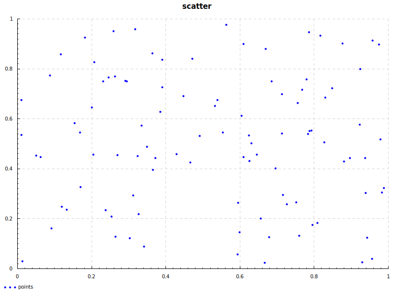
{-# LANGUAGE OverloadedStrings #-}

import qualified DataFrame as D
import qualified Graphics.Rendering.Chart.Backend.Cairo as Cairo
import Graphics.Rendering.Chart.Easy ((.=))
import qualified Graphics.Rendering.Chart.Easy as Chart

chartScatter :: D.DataFrame -> IO ()
chartScatter df =
  let xs = D.extractNumericColumn "x" df
      ys = D.extractNumericColumn "y" df
   in Cairo.toFile Chart.def "plots/chartScatter.png" $ do
        Chart.layout_title .= "scatter"
        Chart.plot $ Chart.points "points" (zip xs ys)

matplotlib (Haskell)

I didn’t mention this in the list above because I decided not to include it, but it is out there:

readData (x, y)
  % mp # "p = plot.plot(data[" # a # "], data[" # b # "]" ## ")"
  % mp # "plot.xlabel(" # str label # ")"

That doesn’t count as not writing Python! That’s just writing Python without any of the development conveniences of writing Python! I’m sure it’s fine. It seems nice to be able to use all of Python’s matplotlib, but writing Python in Haskell felt against the spirit of the exercise.

Other posts in this series

I’ll update this list as I complete the other posts, but here’s the basic outline:

• Hello, plots (this post)
• Plot configuration (titles, axes, axis labels, axis scaling)
• Low-level plotting (annotating plots, drawing shapes wherever you want)